Finite Hankel SISO model reduction

Tutorial goal

Build a finite Hankel matrix from a stable IIR impulse response and construct lower-order rational models with the C++ backend.

Note

New to the terminology? See the lattice DSP concept map and the causality/data-use guide for how online, offline, block, and MIMO examples should be read.

Context

This tutorial is the first executable bridge between the model-reduction theory page and the package API. It is deliberately finite-dimensional: a truncated Hankel matrix is built from the impulse response, its singular values are inspected, and a lower-order Ho–Kalman realization is recovered from the leading Hankel factors.

Exact AAK/Nehari theory is an infinite-dimensional optimal rational-approximation theory. The implementation here is a practical finite-section reducer inspired by the same Hankel-operator viewpoint, but it does not claim exact Nehari or AAK optimality.

Key idea and equations

Given an impulse response h[n], the finite Hankel matrix is

\[H_{ij}=h[i+j+1].\]

Its singular values measure input-output memory. A reduced order r keeps the leading singular directions and forms a balanced finite realization

\[H_0 \approx U_r \Sigma_r V_r^T, \qquad A_r = \Sigma_r^{-1/2}U_r^T H_1 V_r\Sigma_r^{-1/2}.\]

How to read the result

Look for Hankel singular-value decay, retained Hankel energy, impulse-response error, and whether the reduced denominator remains stable.

Run command

python examples/finite_hankel_model_reduction.py

Run status

Return code: 0

Captured stdout

full order: 8
finite Hankel matrix: 48 x 48
leading Hankel singular values: [7.372965, 0.174286, 0.135451, 0.113361, 0.015519, 0.01479, 0.009059, 0.002232]
order=2: stable=True, retained_energy=0.999417, rel_impulse_error=4.282e-03, max_mag_error=1.933 dB
order=4: stable=True, retained_energy=0.999990, rel_impulse_error=3.880e-05, max_mag_error=0.175 dB
order=6: stable=True, retained_energy=0.999998, rel_impulse_error=1.834e-05, max_mag_error=0.129 dB
order=8: stable=True, retained_energy=1.000000, rel_impulse_error=1.115e-23, max_mag_error=0.000 dB

Figures

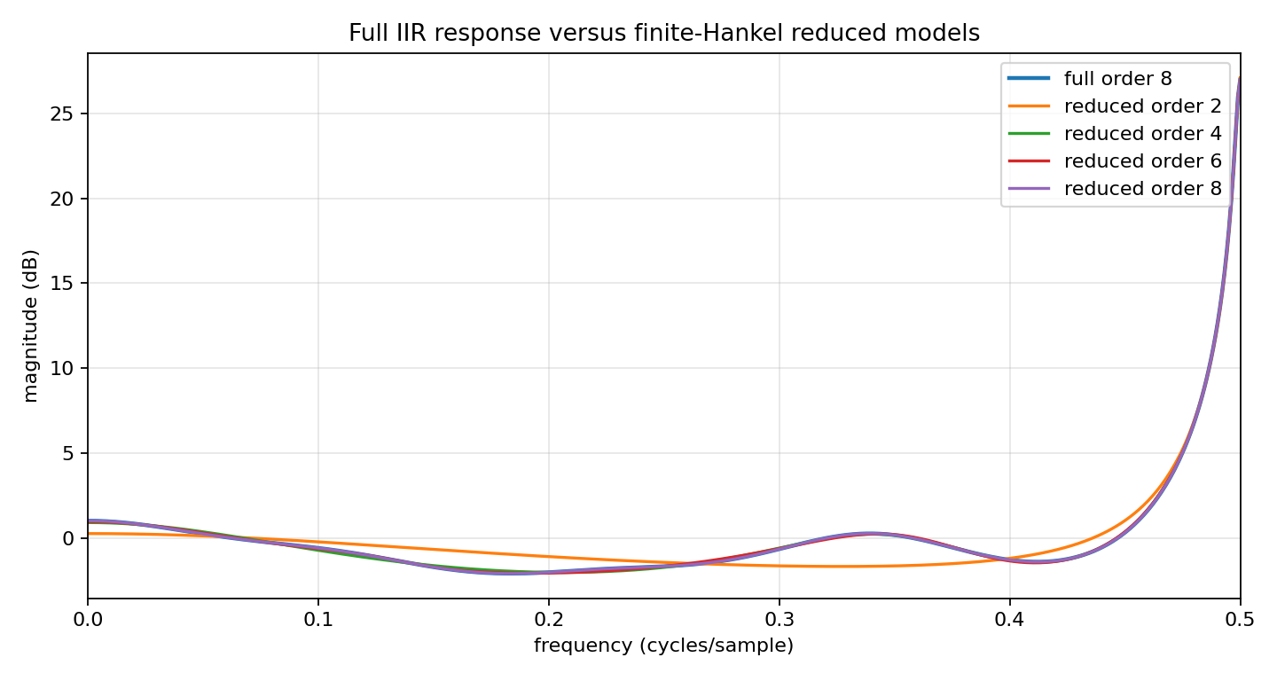
finite_hankel_reduced_responses.png

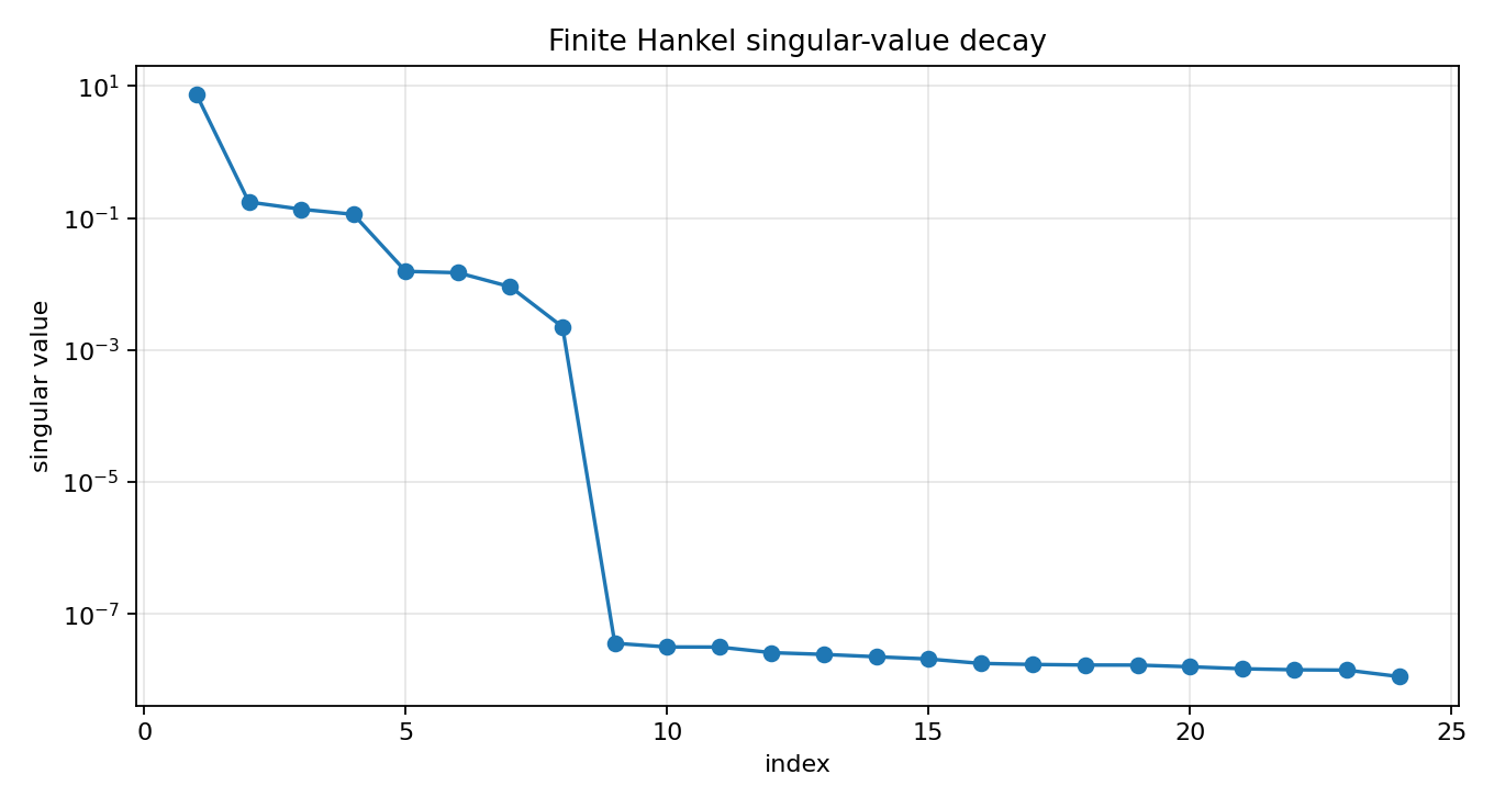
finite_hankel_singular_values.png

Generated data files

• finite_hankel_model_reduction_summary.csv

Source code

"""Tutorial: finite Hankel model reduction for a stable SISO IIR.

This example is a practical bridge between the theory page and executable code.
It builds a stable high-order lattice IIR, forms a finite Hankel matrix from its
impulse response, inspects the Hankel singular values, and constructs lower-order
finite-Hankel reduced models with the C++ backend.

The implementation is intentionally labeled "finite-Hankel/Ho-Kalman": it uses a
truncated Hankel matrix and a Ho-Kalman realization, so it is a useful numerical
approximation and diagnostic rather than a claim of exact infinite-dimensional
AAK or Nehari optimality.
"""

from __future__ import annotations

import csv
import os
from pathlib import Path

import numpy as np

import lattice_dsp as ld


def artifact_dir() -> Path:
    path = Path(os.environ.get("LATTICE_DSP_ARTIFACT_DIR", "reports/example-artifacts"))
    path.mkdir(parents=True, exist_ok=True)
    return path


def freq_response(
    denominator: np.ndarray, numerator: np.ndarray, n_fft: int = 1024
) -> tuple[np.ndarray, np.ndarray]:
    freq = np.linspace(0.0, 0.5, n_fft // 2 + 1)
    z = np.exp(-2j * np.pi * freq)
    num = np.zeros_like(z, dtype=complex)
    den = np.zeros_like(z, dtype=complex)
    for i, coef in enumerate(numerator):
        num += float(coef) * z**i
    for i, coef in enumerate(denominator):
        den += float(coef) * z**i
    mag_db = 20.0 * np.log10(np.maximum(np.abs(num / den), 1e-12))
    return freq, mag_db


def write_summary(path: Path, rows: list[dict[str, float | int | str | bool]]) -> None:
    with path.open("w", newline="", encoding="utf-8") as f:
        fieldnames = [
            "order",
            "stable",
            "retained_hankel_energy",
            "relative_impulse_error",
            "max_magnitude_error_db",
        ]
        writer = csv.DictWriter(f, fieldnames=fieldnames)
        writer.writeheader()
        writer.writerows(rows)


def main() -> None:
    out_dir = artifact_dir()

    # A stable eighth-order all-pole denominator.  In a lattice representation,
    # stability is controlled by |k_i| < 1.
    reflection = np.array([0.62, -0.48, 0.36, -0.28, 0.20, -0.14, 0.09, -0.05], dtype=float)
    numerator = np.array([1.0, -0.22, 0.15, 0.08, -0.05, 0.03, 0.0, 0.0, 0.0], dtype=float)
    denominator = np.asarray(ld.reflection_to_denominator(reflection), dtype=float)

    n_impulse = 360
    rows = cols = 48
    impulse = np.asarray(ld.iir_impulse_response(denominator, numerator, n_impulse), dtype=float)
    hsv = np.asarray(ld.hankel_singular_values(impulse, rows, cols), dtype=float)

    freq, full_mag = freq_response(denominator, numerator)

    orders = [2, 4, 6, 8]
    summary: list[dict[str, float | int | str | bool]] = []
    reduced_curves: dict[int, np.ndarray] = {}

    for order in orders:
        result = ld.finite_hankel_reduce_iir(
            reflection.tolist(),
            numerator.tolist(),
            reduced_order=order,
            n_impulse=n_impulse,
            rows=rows,
            cols=cols,
        )
        red_den = np.asarray(result["denominator"], dtype=float)
        red_num = np.asarray(result["numerator"], dtype=float)
        _, red_mag = freq_response(red_den, red_num)
        reduced_curves[order] = red_mag
        max_mag_err = float(np.max(np.abs(full_mag - red_mag)))
        summary.append(
            {
                "order": order,
                "stable": bool(result["stable"]),
                "retained_hankel_energy": float(result["retained_hankel_energy"]),
                "relative_impulse_error": float(result["relative_impulse_error"]),
                "max_magnitude_error_db": max_mag_err,
            }
        )

    csv_path = out_dir / "finite_hankel_model_reduction_summary.csv"
    write_summary(csv_path, summary)

    print("full order:", len(reflection))
    print("finite Hankel matrix:", f"{rows} x {cols}")
    print("leading Hankel singular values:", [round(float(v), 6) for v in hsv[:8]])
    for row in summary:
        print(
            "order={order}: stable={stable}, retained_energy={retained_hankel_energy:.6f}, "
            "rel_impulse_error={relative_impulse_error:.3e}, max_mag_error={max_magnitude_error_db:.3f} dB".format(
                **row
            )
        )
    print(f"wrote {csv_path}")

    try:
        import matplotlib.pyplot as plt
    except Exception:
        print("matplotlib is not installed; skipped figures")
        return

    fig, ax = plt.subplots(figsize=(8.5, 4.6))
    idx = np.arange(1, min(24, hsv.size) + 1)
    ax.semilogy(idx, hsv[: idx.size], marker="o")
    ax.set_title("Finite Hankel singular-value decay")
    ax.set_xlabel("index")
    ax.set_ylabel("singular value")
    ax.grid(True, alpha=0.3)
    fig.tight_layout()
    fig_path = out_dir / "finite_hankel_singular_values.png"
    fig.savefig(fig_path, dpi=160)
    print(f"wrote {fig_path}")

    fig2, ax2 = plt.subplots(figsize=(9, 4.8))
    ax2.plot(freq, full_mag, linewidth=2.0, label="full order 8")
    for order in orders:
        ax2.plot(freq, reduced_curves[order], label=f"reduced order {order}")
    ax2.set_title("Full IIR response versus finite-Hankel reduced models")
    ax2.set_xlabel("frequency (cycles/sample)")
    ax2.set_ylabel("magnitude (dB)")
    ax2.set_xlim(0.0, 0.5)
    ax2.grid(True, alpha=0.3)
    ax2.legend()
    fig2.tight_layout()
    fig2_path = out_dir / "finite_hankel_reduced_responses.png"
    fig2.savefig(fig2_path, dpi=160)
    print(f"wrote {fig2_path}")


if __name__ == "__main__":
    main()