LMS through the H-infinity lens
Tutorial goal
Reproduce the qualitative message of Hassibi–Sayed–Kailath: LMS is not only crude least-squares descent; it also has a worst-case energy-gain interpretation.
Note
New to the terminology? See the lattice DSP concept map and the causality/data-use guide for how online, offline, block, and MIMO examples should be read.
Context
This flagship tutorial explains a historical surprise in adaptive filtering. The LMS idea goes back to Widrow and Hoff’s 1960 adaptive switching work. For more than three decades, it was often introduced as the inexpensive stochastic-gradient approximation to least squares, while RLS was the exact least-squares recursion. Hassibi, Sayed, and Kailath then showed that LMS also has a deterministic robust-filtering interpretation: with the right viewpoint, the algorithm is tied to an H-infinity minimax energy-gain problem rather than only to an average squared-error objective.
That historical angle is useful because it changes the way readers interpret a familiar algorithm. The script below does not try to reprint every derivation from the 1996 paper. Instead it builds a finite-horizon diagnostic that readers can inspect: for fixed regressors, the map from additive disturbance to prediction error is a linear operator. Its largest singular value exposes the disturbance direction that causes the largest error-energy amplification.
Key idea and equations
The adaptive filtering model is
where u_i is the regressor, w_* is the unknown vector, and v_i is a disturbance.
Least-squares thinking focuses on sums such as
The robust H-infinity diagnostic instead asks for a worst-case energy gain. In this tutorial we estimate, for each algorithm,
by forming the finite-horizon sensitivity matrix from disturbance samples to noise-induced prediction errors.
How to read the result
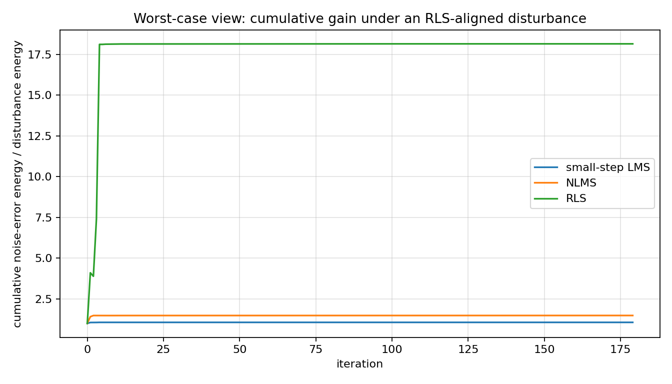
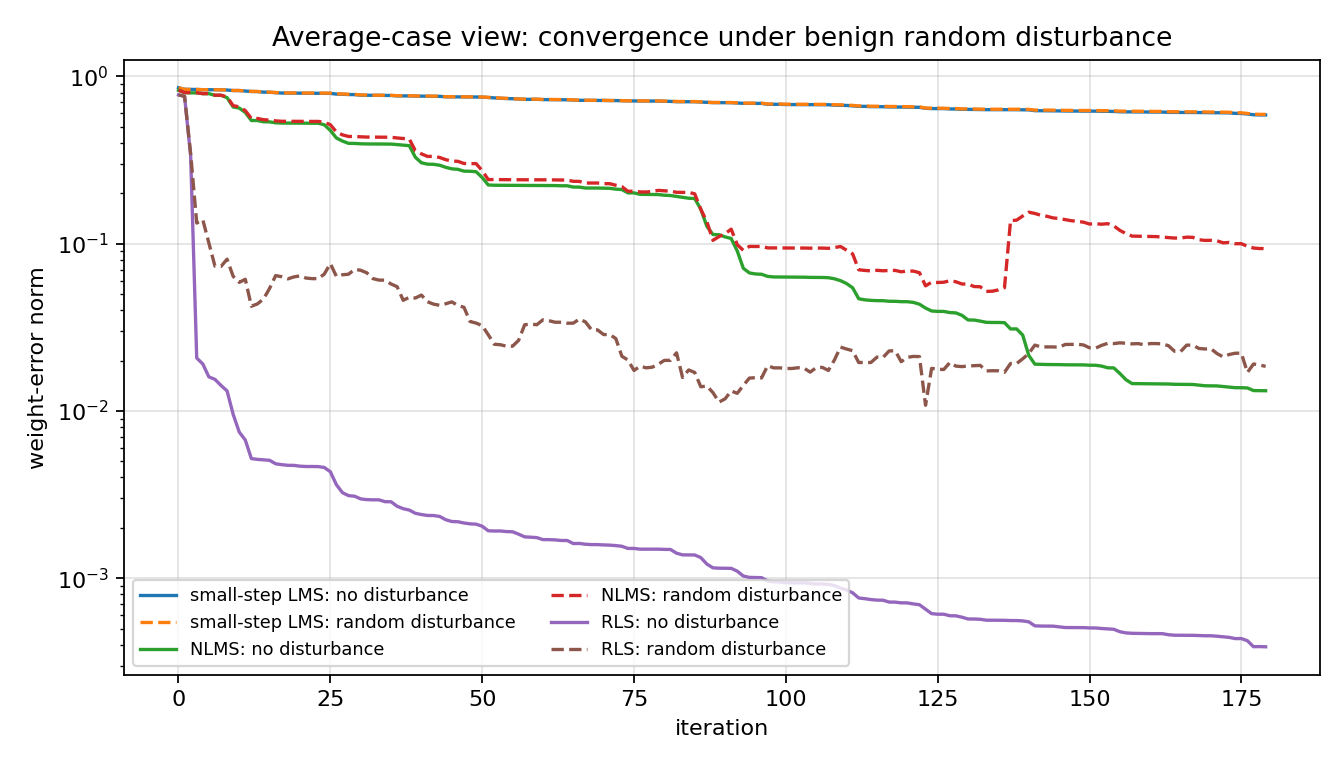
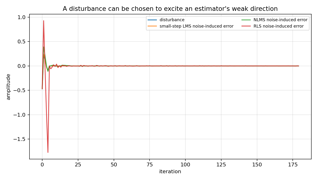
Read the first plot in the classical least-squares way: RLS converges fastest under benign random noise. Then read the gain plots in the minimax way: the same estimator can have a larger worst-case disturbance direction. That change of viewpoint is the lesson.
Run command
python examples/hinf_lms_reproduction.py
Run status
Return code: 0
Captured stdout
H-infinity-inspired LMS/RLS diagnostic
samples=180, order=4, noise_rms=0.04

algorithm            worst gain  random gain  RLS-worst gain  random tail MSE
----------------------------------------------------------------------------------
small-step LMS            2.568        1.052           1.064        3.016e-02
NLMS                     15.040        1.539           1.486        3.900e-03
RLS                      18.152        1.219          18.152        1.498e-03

Interpretation:
  RLS usually converges fastest under benign random noise, but the sensitivity
  matrix exposes directions where disturbance energy is amplified more strongly.
  Small-step LMS is slower, yet its disturbance-to-error gain can be smaller.
  This illustrates the Hassibi-Sayed-Kailath message: LMS can be understood
  through a worst-case energy-gain lens, not only as crude least-squares descent.
Figures
hinf_lms_cumulative_gain.png
hinf_lms_random_convergence.png
hinf_lms_worst_case_disturbance.png
Generated data files
Source code
  1from __future__ import annotations
  2
  3import csv
  4import os
  5from dataclasses import dataclass
  6from pathlib import Path
  7
  8import matplotlib.pyplot as plt
  9import numpy as np
 10
 11
 12@dataclass(frozen=True)
 13class Algorithm:
 14    name: str
 15    kind: str
 16    mu: float = 0.0
 17    lam: float = 0.995
 18    p0: float = 100.0
 19    eps: float = 1e-6
 20
 21
 22def artifact_dir() -> Path:
 23    path = Path(os.environ.get("LATTICE_DSP_ARTIFACT_DIR", "reports/example-artifacts"))
 24    path.mkdir(parents=True, exist_ok=True)
 25    return path
 26
 27
 28def make_regressors(n: int = 180, order: int = 4, seed: int = 12) -> np.ndarray:
 29    rng = np.random.default_rng(seed)
 30    x = rng.normal(size=n + order + 2)
 31    for i in range(1, len(x)):
 32        x[i] = 0.92 * x[i - 1] + 0.45 * x[i]
 33    u = np.zeros((n, order), dtype=float)
 34    for i in range(n):
 35        u[i] = x[i + order - 1 : i - 1 : -1] if i > 0 else x[order - 1 :: -1]
 36    return u / np.sqrt(np.mean(u * u))
 37
 38
 39def run_adaptive(
 40    u: np.ndarray, w_true: np.ndarray, disturbance: np.ndarray, alg: Algorithm
 41) -> dict[str, np.ndarray]:
 42    n, p = u.shape
 43    w = np.zeros(p, dtype=float)
 44    P = alg.p0 * np.eye(p)
 45
 46    pred_error = np.zeros(n)
 47    posterior_error = np.zeros(n)
 48    weight_error = np.zeros(n)
 49    weights = np.zeros((n, p))
 50
 51    for i, ui in enumerate(u):
 52        d = float(ui @ w_true + disturbance[i])
 53        e = d - float(ui @ w)
 54        pred_error[i] = e
 55
 56        if alg.kind == "lms":
 57            w = w + alg.mu * ui * e
 58        elif alg.kind == "nlms":
 59            w = w + (alg.mu / (alg.eps + float(ui @ ui))) * ui * e
 60        elif alg.kind == "rls":
 61            Pu = P @ ui
 62            gain = Pu / (alg.lam + float(ui @ Pu))
 63            w = w + gain * e
 64            P = (P - np.outer(gain, ui) @ P) / alg.lam
 65            P = 0.5 * (P + P.T)
 66        else:
 67            raise ValueError(f"Unknown algorithm kind: {alg.kind}")
 68
 69        posterior_error[i] = d - float(ui @ w)
 70        weight_error[i] = np.linalg.norm(w - w_true)
 71        weights[i] = w
 72
 73    return {
 74        "prediction_error": pred_error,
 75        "posterior_error": posterior_error,
 76        "weight_error": weight_error,
 77        "weights": weights,
 78    }
 79
 80
 81def sensitivity_matrix(
 82    u: np.ndarray, w_true: np.ndarray, alg: Algorithm, *, output: str
 83) -> tuple[np.ndarray, float, np.ndarray]:
 84    n = u.shape[0]
 85    zero = np.zeros(n)
 86    base = run_adaptive(u, w_true, zero, alg)[output]
 87    M = np.zeros((n, n), dtype=float)
 88    for j in range(n):
 89        impulse = np.zeros(n)
 90        impulse[j] = 1.0
 91        response = run_adaptive(u, w_true, impulse, alg)[output]
 92        M[:, j] = response - base
 93    U, S, Vt = np.linalg.svd(M, full_matrices=False)
 94    return M, float(S[0] ** 2), Vt[0]
 95
 96
 97def cumulative_gain(noise_error: np.ndarray, disturbance: np.ndarray) -> np.ndarray:
 98    num = np.cumsum(noise_error * noise_error)
 99    den = np.cumsum(disturbance * disturbance) + 1e-30
100    return num / den
101
102
103def main() -> None:
104    out_dir = artifact_dir()
105    rng = np.random.default_rng(4)
106
107    n = 180
108    order = 4
109    u = make_regressors(n=n, order=order)
110    w_true = np.array([0.70, -0.42, 0.25, -0.12])
111    noise_rms = 0.04
112
113    algorithms = [
114        Algorithm("small-step LMS", "lms", mu=0.020),
115        Algorithm("NLMS", "nlms", mu=0.25),
116        Algorithm("RLS", "rls", lam=0.995, p0=100.0),
117    ]
118
119    random_disturbance = noise_rms * rng.normal(size=n)
120
121    sensitivity: dict[str, dict[str, object]] = {}
122    for alg in algorithms:
123        M, gain, v_unit = sensitivity_matrix(u, w_true, alg, output="prediction_error")
124        sensitivity[alg.name] = {"matrix": M, "gain": gain, "v_unit": v_unit}
125
126    # Worst-case disturbance for the RLS prediction-error map.  Scale it to the same
127    # energy as a length-n Gaussian sequence with RMS = noise_rms.
128    rls_worst_unit = np.asarray(sensitivity["RLS"]["v_unit"], dtype=float)
129    rls_worst_disturbance = noise_rms * np.sqrt(n) * rls_worst_unit
130
131    zero = np.zeros(n)
132    rows = []
133    trajectories: dict[str, dict[str, dict[str, np.ndarray]]] = {}
134
135    for alg in algorithms:
136        clean = run_adaptive(u, w_true, zero, alg)
137        random_run = run_adaptive(u, w_true, random_disturbance, alg)
138        worst_run = run_adaptive(u, w_true, rls_worst_disturbance, alg)
139
140        random_noise_error = random_run["prediction_error"] - clean["prediction_error"]
141        worst_noise_error = worst_run["prediction_error"] - clean["prediction_error"]
142
143        rows.append(
144            {
145                "algorithm": alg.name,
146                "mu_or_lambda": alg.mu if alg.kind != "rls" else alg.lam,
147                "operator_worst_case_gain": float(sensitivity[alg.name]["gain"]),
148                "random_noise_gain": float(
149                    np.sum(random_noise_error**2) / (np.sum(random_disturbance**2) + 1e-30)
150                ),
151                "rls_worst_disturbance_gain": float(
152                    np.sum(worst_noise_error**2) / (np.sum(rls_worst_disturbance**2) + 1e-30)
153                ),
154                "clean_final_weight_error": float(clean["weight_error"][-1]),
155                "random_final_weight_error": float(random_run["weight_error"][-1]),
156                "rls_worst_final_weight_error": float(worst_run["weight_error"][-1]),
157                "random_tail_mse": float(np.mean(random_run["prediction_error"][-50:] ** 2)),
158                "rls_worst_tail_mse": float(np.mean(worst_run["prediction_error"][-50:] ** 2)),
159            }
160        )
161        trajectories[alg.name] = {"clean": clean, "random": random_run, "rls_worst": worst_run}
162
163    csv_path = out_dir / "hinf_lms_summary.csv"
164    with csv_path.open("w", newline="", encoding="utf-8") as f:
165        writer = csv.DictWriter(f, fieldnames=list(rows[0].keys()))
166        writer.writeheader()
167        writer.writerows(rows)
168
169    t = np.arange(n)
170
171    fig, ax = plt.subplots(figsize=(8.4, 4.8))
172    for alg in algorithms:
173        ax.semilogy(
174            t, trajectories[alg.name]["clean"]["weight_error"], label=f"{alg.name}: no disturbance"
175        )
176        ax.semilogy(
177            t,
178            trajectories[alg.name]["random"]["weight_error"],
179            linestyle="--",
180            label=f"{alg.name}: random disturbance",
181        )
182    ax.set_title("Average-case view: convergence under benign random disturbance")
183    ax.set_xlabel("iteration")
184    ax.set_ylabel("weight-error norm")
185    ax.grid(True, alpha=0.35)
186    ax.legend(ncol=2, fontsize=8)
187    fig.tight_layout()
188    convergence_path = out_dir / "hinf_lms_random_convergence.png"
189    fig.savefig(convergence_path, dpi=160)
190    plt.close(fig)
191
192    fig, ax = plt.subplots(figsize=(8.4, 4.8))
193    for alg in algorithms:
194        clean = trajectories[alg.name]["clean"]
195        worst = trajectories[alg.name]["rls_worst"]
196        noise_error = worst["prediction_error"] - clean["prediction_error"]
197        ax.plot(t, cumulative_gain(noise_error, rls_worst_disturbance), label=alg.name)
198    ax.set_title("Worst-case view: cumulative gain under an RLS-aligned disturbance")
199    ax.set_xlabel("iteration")
200    ax.set_ylabel("cumulative noise-error energy / disturbance energy")
201    ax.grid(True, alpha=0.35)
202    ax.legend()
203    fig.tight_layout()
204    gain_path = out_dir / "hinf_lms_cumulative_gain.png"
205    fig.savefig(gain_path, dpi=160)
206    plt.close(fig)
207
208    fig, ax = plt.subplots(figsize=(8.4, 4.8))
209    ax.plot(t, rls_worst_disturbance, label="disturbance")
210    for alg in algorithms:
211        clean = trajectories[alg.name]["clean"]
212        worst = trajectories[alg.name]["rls_worst"]
213        noise_error = worst["prediction_error"] - clean["prediction_error"]
214        ax.plot(t, noise_error, label=f"{alg.name} noise-induced error", alpha=0.85)
215    ax.set_title("A disturbance can be chosen to excite an estimator's weak direction")
216    ax.set_xlabel("iteration")
217    ax.set_ylabel("amplitude")
218    ax.grid(True, alpha=0.35)
219    ax.legend(fontsize=8, ncol=2)
220    fig.tight_layout()
221    disturbance_path = out_dir / "hinf_lms_worst_case_disturbance.png"
222    fig.savefig(disturbance_path, dpi=160)
223    plt.close(fig)
224
225    print("H-infinity-inspired LMS/RLS diagnostic")
226    print(f"samples={n}, order={order}, noise_rms={noise_rms}")
227    print()
228    print(
229        f"{'algorithm':18s} {'worst gain':>12s} {'random gain':>12s} {'RLS-worst gain':>15s} {'random tail MSE':>16s}"
230    )
231    print("-" * 82)
232    for row in rows:
233        print(
234            f"{row['algorithm']:18s} "
235            f"{row['operator_worst_case_gain']:12.3f} "
236            f"{row['random_noise_gain']:12.3f} "
237            f"{row['rls_worst_disturbance_gain']:15.3f} "
238            f"{row['random_tail_mse']:16.3e}"
239        )
240    print()
241    print("Interpretation:")
242    print("  RLS usually converges fastest under benign random noise, but the sensitivity")
243    print("  matrix exposes directions where disturbance energy is amplified more strongly.")
244    print("  Small-step LMS is slower, yet its disturbance-to-error gain can be smaller.")
245    print("  This illustrates the Hassibi-Sayed-Kailath message: LMS can be understood")
246    print("  through a worst-case energy-gain lens, not only as crude least-squares descent.")
247    print()
248    print(f"Wrote {convergence_path}")
249    print(f"Wrote {gain_path}")
250    print(f"Wrote {disturbance_path}")
251    print(f"Wrote {csv_path}")
252
253
254if __name__ == "__main__":
255    main()