Spectral diagnostics comparison and tuning

Tutorial goal

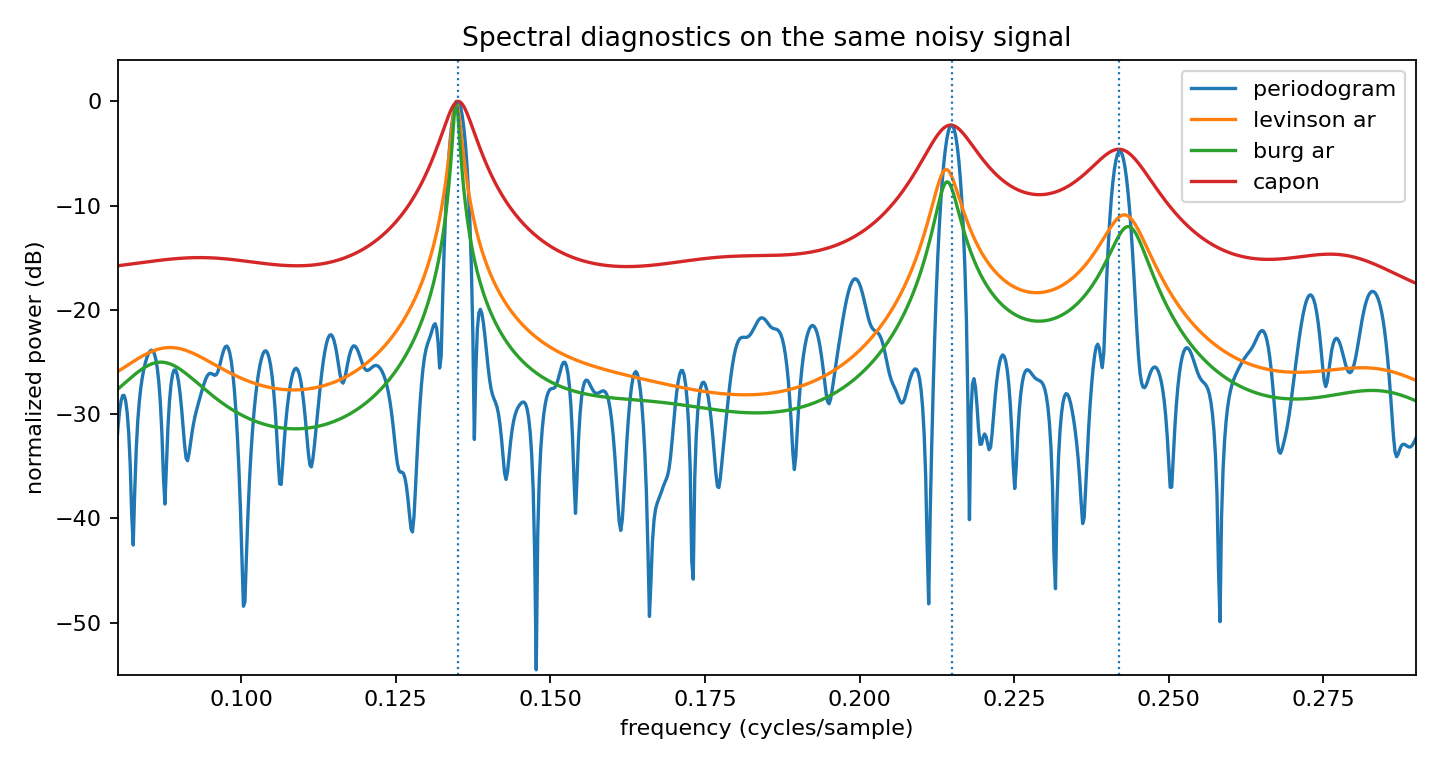
Compare periodogram, AR, Burg, and Capon spectra, then vary model order/aperture.

Note

New to the terminology? See the lattice DSP concept map and the causality/data-use guide for how online, offline, block, and MIMO examples should be read.

Context

This is the tutorial page to read after the two focused spectral examples. It keeps the signal fixed and changes the diagnostic method or its tuning parameter so the reader can see how visual conclusions depend on modeling choices.

Key idea and equations

The tunable quantities are model complexity parameters: AR order p and Capon aperture M. Larger values can increase resolution, but they can also amplify finite-sample noise.

How to read the result

Use the second figure as a tuning guide: peaks should align with true tones, but excessive sharpness or spurious peaks are a warning sign.

Run command

python examples/spectral_diagnostics_comparison.py

Run status

Return code: 0

Captured stdout

true tone frequencies: [0.135, 0.215, 0.242]
main AR order: 24
main Capon aperture: 36

Figures

spectral_diagnostics_comparison.png

spectral_diagnostics_tuning.png

Generated data files

• spectral_diagnostics_comparison.csv

Source code

"""Tutorial: compare spectral diagnostics as the model complexity changes.

This example places periodogram, AR, and Capon estimates on the same synthetic
signal, then adds a second figure showing how AR model order and Capon aperture
change the diagnostic.  It is meant as a visual tuning guide rather than a new
API surface.
"""

from __future__ import annotations

import csv
import os
from pathlib import Path

import numpy as np

from lattice_dsp import autocorrelation, burg_denominator, levinson_durbin_denominator


def artifact_dir() -> Path:
    path = Path(os.environ.get("LATTICE_DSP_ARTIFACT_DIR", "reports/example-artifacts"))
    path.mkdir(parents=True, exist_ok=True)
    return path


def db_normalized(power: np.ndarray) -> np.ndarray:
    power = np.maximum(np.asarray(power, dtype=float), 1e-18)
    return 10.0 * np.log10(power / np.max(power))


def periodogram(x: np.ndarray, n_fft: int) -> tuple[np.ndarray, np.ndarray]:
    window = np.hanning(x.size)
    spectrum = np.fft.rfft(window * x, n=n_fft)
    return np.fft.rfftfreq(n_fft), np.abs(spectrum) ** 2 / max(np.sum(window**2), 1e-12)


def ar_spectrum(denominator: np.ndarray, freq: np.ndarray) -> np.ndarray:
    z = np.exp(-2j * np.pi * freq)
    a = np.zeros_like(z, dtype=complex)
    for i, coef in enumerate(denominator):
        a += float(coef) * z**i
    return 1.0 / np.maximum(np.abs(a) ** 2, 1e-18)


def capon_spectrum(x: np.ndarray, aperture: int, freq: np.ndarray) -> np.ndarray:
    windows = np.lib.stride_tricks.sliding_window_view(x, aperture).astype(complex)
    R = (windows.conj().T @ windows) / windows.shape[0]
    loading = 1e-3 * float(np.trace(R).real) / aperture
    Rinv = np.linalg.pinv(R + loading * np.eye(aperture))
    n = np.arange(aperture)
    out = np.empty_like(freq, dtype=float)
    for i, f in enumerate(freq):
        steering = np.exp(-2j * np.pi * f * n)
        out[i] = 1.0 / max(np.vdot(steering, Rinv @ steering).real, 1e-18)
    return out


def write_csv(path: Path, freq: np.ndarray, columns: dict[str, np.ndarray]) -> None:
    with path.open("w", newline="", encoding="utf-8") as f:
        writer = csv.writer(f)
        writer.writerow(["frequency_cycles_per_sample", *columns])
        for i, value in enumerate(freq):
            writer.writerow([value, *(columns[name][i] for name in columns)])


def main() -> None:
    rng = np.random.default_rng(909)
    samples = 640
    n = np.arange(samples)
    tones = [0.135, 0.215, 0.242]
    x = (
        1.0 * np.sin(2 * np.pi * tones[0] * n + 0.2)
        + 0.75 * np.sin(2 * np.pi * tones[1] * n)
        + 0.65 * np.sin(2 * np.pi * tones[2] * n + 1.2)
        + 0.50 * rng.normal(size=samples)
    )
    x -= np.mean(x)

    n_fft = 4096
    freq, p_per = periodogram(x, n_fft)

    order = 24
    den_ld = np.asarray(levinson_durbin_denominator(autocorrelation(x, order), order), dtype=float)
    den_burg = np.asarray(burg_denominator(x, order), dtype=float)
    p_ld = ar_spectrum(den_ld, freq)
    p_burg = ar_spectrum(den_burg, freq)
    p_capon = capon_spectrum(x, 36, freq)

    out_dir = artifact_dir()
    columns = {
        "periodogram_db": db_normalized(p_per),
        "levinson_ar_db": db_normalized(p_ld),
        "burg_ar_db": db_normalized(p_burg),
        "capon_db": db_normalized(p_capon),
    }
    csv_path = out_dir / "spectral_diagnostics_comparison.csv"
    write_csv(csv_path, freq, columns)

    print("true tone frequencies:", tones)
    print("main AR order:", order)
    print("main Capon aperture:", 36)
    print(f"wrote {csv_path}")

    try:
        import matplotlib.pyplot as plt
    except Exception:
        print("matplotlib is not installed; skipped figures")
        return

    fig, ax = plt.subplots(figsize=(9, 4.8))
    for name, values in columns.items():
        label = name.replace("_db", "").replace("_", " ")
        ax.plot(freq, values, label=label)
    for tone in tones:
        ax.axvline(tone, linestyle=":", linewidth=1.0)
    ax.set_xlim(0.08, 0.29)
    ax.set_ylim(-55, 4)
    ax.set_title("Spectral diagnostics on the same noisy signal")
    ax.set_xlabel("frequency (cycles/sample)")
    ax.set_ylabel("normalized power (dB)")
    ax.legend()
    fig.tight_layout()
    fig_path = out_dir / "spectral_diagnostics_comparison.png"
    fig.savefig(fig_path, dpi=160)
    print(f"wrote {fig_path}")

    fig2, ax2 = plt.subplots(figsize=(9, 4.8))
    for test_order in [8, 16, 32]:
        den = np.asarray(
            levinson_durbin_denominator(autocorrelation(x, test_order), test_order), dtype=float
        )
        ax2.plot(freq, db_normalized(ar_spectrum(den, freq)), label=f"AR order {test_order}")
    for aperture in [20, 44]:
        ax2.plot(
            freq,
            db_normalized(capon_spectrum(x, aperture, freq)),
            linestyle="--",
            label=f"Capon aperture {aperture}",
        )
    for tone in tones:
        ax2.axvline(tone, linestyle=":", linewidth=1.0)
    ax2.set_xlim(0.08, 0.29)
    ax2.set_ylim(-55, 4)
    ax2.set_title("Changing AR order and Capon aperture changes the diagnostic")
    ax2.set_xlabel("frequency (cycles/sample)")
    ax2.set_ylabel("normalized power (dB)")
    ax2.legend(ncol=2)
    fig2.tight_layout()
    fig2_path = out_dir / "spectral_diagnostics_tuning.png"
    fig2.savefig(fig2_path, dpi=160)
    print(f"wrote {fig2_path}")


if __name__ == "__main__":
    main()