Finite block-Hankel MIMO model reduction

Tutorial goal

Generalize the SISO finite-Hankel reducer to MIMO Markov matrices and return a reduced state-space model.

Note

New to the terminology? See the lattice DSP concept map and the causality/data-use guide for how online, offline, block, and MIMO examples should be read.

Context

The SISO reducer works with one impulse response. A MIMO system has a sequence of Markov matrices instead, where each matrix maps input channels to output channels at a particular lag. The natural finite-Hankel baseline is therefore a block-Hankel matrix.

This tutorial is deliberately a baseline: it gives a reference MIMO Ho–Kalman/ERA-style reduction as a finite block-Hankel baseline separate from matrix Nehari or AAK optimality claims.

Key idea and equations

For Markov matrices M_k with shape outputs x inputs, the finite block-Hankel matrix is

\[\begin{split}\mathcal{H}_0 = \begin{bmatrix} M_1 & M_2 & M_3 & \cdots \\ M_2 & M_3 & M_4 & \cdots \\ M_3 & M_4 & M_5 & \cdots \\ \vdots & \vdots & \vdots & \ddots \end{bmatrix}.\end{split}\]

The reduced model is returned as state-space matrices A, B, C, D rather than as scalar numerator/denominator coefficients.

How to read the result

Look for block-Hankel singular-value decay, retained energy, Markov-response error, and stable reduced state matrices.

Run command

python examples/mimo_finite_hankel_model_reduction.py

Run status

Return code: 0

Captured stdout

full state order: 10
inputs: 3 outputs: 3
block Hankel matrix: 72 x 72
leading block-Hankel singular values: [1.314253, 1.043921, 0.377351, 0.26784, 0.108761, 0.028447, 0.012295, 0.000909, 0.000586, 0.000176]
order=2: stable=True, retained_energy=0.925451, relative_markov_error=8.520e-02
order=4: stable=True, retained_energy=0.995798, relative_markov_error=4.148e-03
order=6: stable=True, retained_energy=0.999950, relative_markov_error=6.925e-05

Figures

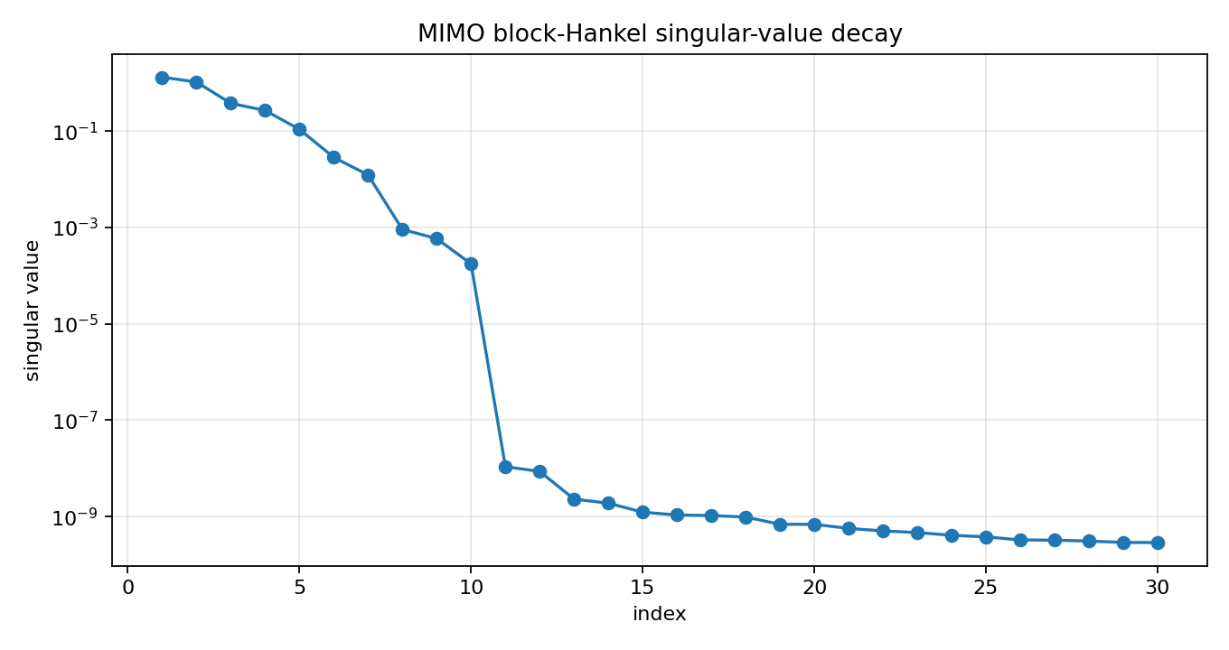
mimo_block_hankel_singular_values.png

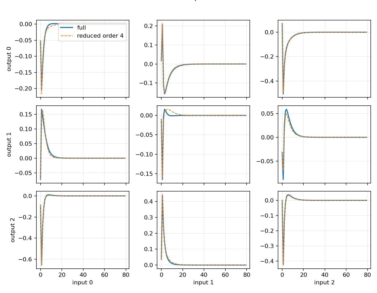
mimo_reduced_markov_responses.png

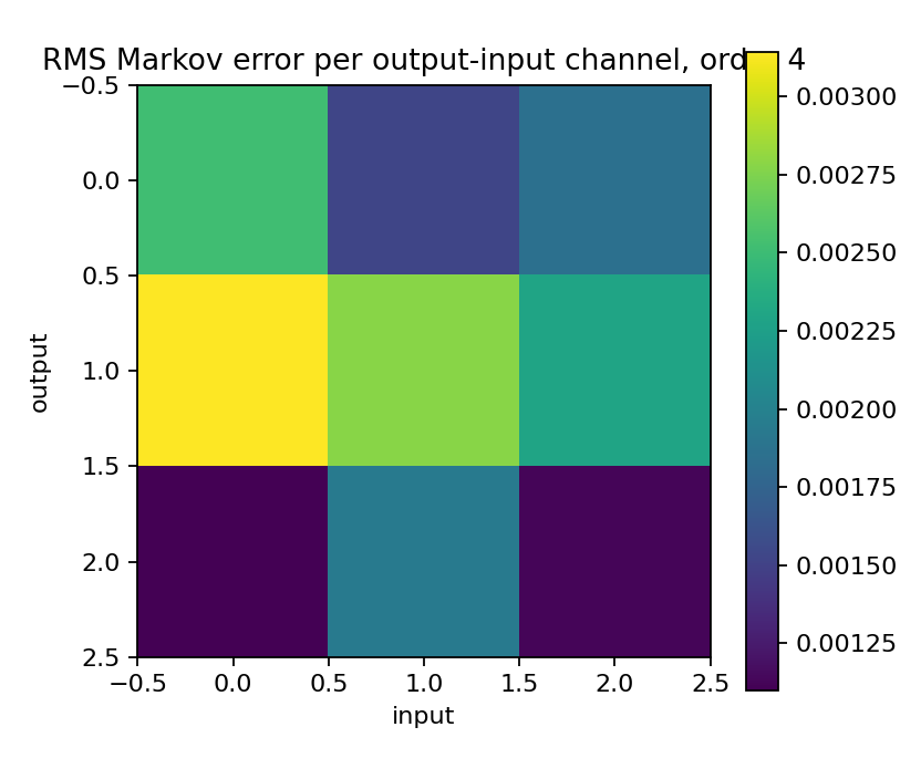
mimo_reduction_error_heatmap.png

Generated data files

• mimo_finite_hankel_model_reduction_summary.csv

Source code

"""Tutorial: finite block-Hankel model reduction for a MIMO system.

The SISO finite-Hankel reducer works with one impulse response.  The MIMO
baseline generalizes this to a sequence of Markov matrices M_k, where each
matrix maps input channels to output channels at lag k.

This tutorial builds a stable coupled 3-input/3-output state-space system,
computes its Markov parameters, performs finite block-Hankel reduction, and
compares the reduced Markov responses against the full system.
"""

from __future__ import annotations

import csv
import os
from pathlib import Path

import numpy as np

import lattice_dsp as ld


def artifact_dir() -> Path:
    path = Path(os.environ.get("LATTICE_DSP_ARTIFACT_DIR", "reports/example-artifacts"))
    path.mkdir(parents=True, exist_ok=True)
    return path


def stable_random_state_space(order: int, outputs: int, inputs: int, seed: int = 7):
    rng = np.random.default_rng(seed)
    q, _ = np.linalg.qr(rng.normal(size=(order, order)))
    radii = np.linspace(0.82, 0.18, order)
    A = q @ np.diag(radii) @ q.T
    B = 0.45 * rng.normal(size=(order, inputs))
    C = 0.45 * rng.normal(size=(outputs, order))
    D = 0.05 * rng.normal(size=(outputs, inputs))
    return A, B, C, D


def main() -> None:
    out_dir = artifact_dir()

    full_order = 10
    inputs = outputs = 3
    n_markov = 180
    block_rows = block_cols = 24
    reduced_orders = [2, 4, 6]

    A, B, C, D = stable_random_state_space(full_order, outputs, inputs)
    markov = ld.mimo_state_space_markov_response(A, B, C, D, n_markov)

    summary = []
    reduced_markov = {}
    for order in reduced_orders:
        result = ld.finite_hankel_reduce_mimo(
            markov,
            reduced_order=order,
            block_rows=block_rows,
            block_cols=block_cols,
        )
        approx = ld.mimo_state_space_markov_response(
            result["A"], result["B"], result["C"], result["D"], n_markov
        )
        rel_error = float(np.sum((markov - approx) ** 2) / np.sum(markov**2))
        reduced_markov[order] = approx
        summary.append(
            {
                "order": order,
                "stable": bool(result["stable"]),
                "retained_hankel_energy": float(result["retained_hankel_energy"]),
                "relative_markov_error": rel_error,
            }
        )

    csv_path = out_dir / "mimo_finite_hankel_model_reduction_summary.csv"
    with csv_path.open("w", newline="", encoding="utf-8") as f:
        writer = csv.DictWriter(f, fieldnames=list(summary[0]))
        writer.writeheader()
        writer.writerows(summary)

    hsv = np.asarray(
        ld.finite_hankel_reduce_mimo(markov, 6, block_rows, block_cols)["hankel_singular_values"]
    )
    print("full state order:", full_order)
    print("inputs:", inputs, "outputs:", outputs)
    print("block Hankel matrix:", f"{block_rows * outputs} x {block_cols * inputs}")
    print("leading block-Hankel singular values:", [round(float(v), 6) for v in hsv[:10]])
    for row in summary:
        print(
            "order={order}: stable={stable}, retained_energy={retained_hankel_energy:.6f}, "
            "relative_markov_error={relative_markov_error:.3e}".format(**row)
        )
    print(f"wrote {csv_path}")

    try:
        import matplotlib.pyplot as plt
    except Exception:
        print("matplotlib is not installed; skipped figures")
        return

    fig, ax = plt.subplots(figsize=(8.5, 4.5))
    idx = np.arange(1, min(30, hsv.size) + 1)
    ax.semilogy(idx, hsv[: idx.size], marker="o")
    ax.set_title("MIMO block-Hankel singular-value decay")
    ax.set_xlabel("index")
    ax.set_ylabel("singular value")
    ax.grid(True, alpha=0.3)
    fig.tight_layout()
    fig_path = out_dir / "mimo_block_hankel_singular_values.png"
    fig.savefig(fig_path, dpi=160)
    print(f"wrote {fig_path}")

    fig2, axes = plt.subplots(outputs, inputs, figsize=(9, 7), sharex=True)
    t = np.arange(80)
    for y in range(outputs):
        for u in range(inputs):
            ax = axes[y, u]
            ax.plot(t, markov[: t.size, y, u], linewidth=1.8, label="full")
            ax.plot(
                t, reduced_markov[4][: t.size, y, u], "--", linewidth=1.2, label="reduced order 4"
            )
            ax.grid(True, alpha=0.25)
            if y == outputs - 1:
                ax.set_xlabel(f"input {u}")
            if u == 0:
                ax.set_ylabel(f"output {y}")
    axes[0, 0].legend(loc="upper right")
    fig2.suptitle("Selected MIMO Markov responses: full vs reduced", y=1.02)
    fig2.tight_layout()
    fig2_path = out_dir / "mimo_reduced_markov_responses.png"
    fig2.savefig(fig2_path, dpi=160)
    print(f"wrote {fig2_path}")

    err = np.sqrt(np.mean((markov - reduced_markov[4]) ** 2, axis=0))
    fig3, ax3 = plt.subplots(figsize=(5.2, 4.4))
    im = ax3.imshow(err)
    ax3.set_title("RMS Markov error per output-input channel, order 4")
    ax3.set_xlabel("input")
    ax3.set_ylabel("output")
    fig3.colorbar(im, ax=ax3)
    fig3.tight_layout()
    fig3_path = out_dir / "mimo_reduction_error_heatmap.png"
    fig3.savefig(fig3_path, dpi=160)
    print(f"wrote {fig3_path}")


if __name__ == "__main__":
    main()