Coupled MIMO finite-Hankel model reduction
Tutorial goal
Reduce a genuinely coupled MIMO state-space system with the finite block-Hankel baseline.
Note
New to the terminology? See the lattice DSP concept map and the causality/data-use guide for how online, offline, block, and MIMO examples should be read.
Context
The diagonal MIMO tutorial shows that independent SISO filters are a special case. This tutorial uses a dense, stable state-space system where each input can affect each output. The goal is to validate the practical MIMO finite-section baseline on a coupled system while keeping it separate from matrix AAK/Nehari algorithms.
The reducer works with Markov matrices and returns a reduced state-space realization. This is the natural representation for MIMO; scalar numerator/denominator coefficients are not forced onto a multivariable system.
Key idea and equations
A coupled MIMO state-space model has
Its Markov matrices are
The finite block-Hankel reducer constructs a reduced model
(A_r,B_r,C_r,D) from the leading singular directions of the block-Hankel matrix.
How to read the result
Look for nonzero off-diagonal channels, block-Hankel singular-value decay, decreasing Markov/output error with order, and reduced state radii below one.
Run command
python examples/mimo_coupled_model_reduction.py
Run status
Return code: 0
Captured stdout
full state order: 12
inputs: 3 outputs: 3
full state spectral radius: 0.8800
block Hankel matrix: 84 x 84
leading block-Hankel singular values: [1.35522, 0.96156, 0.46076, 0.35792, 0.321092, 0.229692, 0.088418, 0.032477, 0.016566, 0.006026]
order=2: stable=True, radius=0.7711, retained=0.845267, markov_error=1.456e-01, output_snr=8.32 dB
order=4: stable=True, radius=0.8338, retained=0.949473, markov_error=5.220e-02, output_snr=12.78 dB
order=6: stable=True, radius=0.8562, retained=0.997184, markov_error=3.630e-03, output_snr=24.45 dB
order=8: stable=True, radius=0.8809, retained=0.999900, markov_error=1.589e-04, output_snr=38.02 dB
Figures
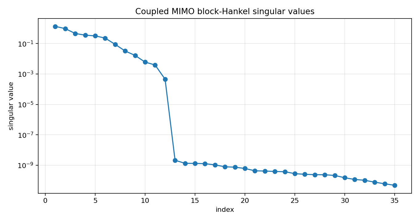
mimo_coupled_block_hankel_singular_values.png
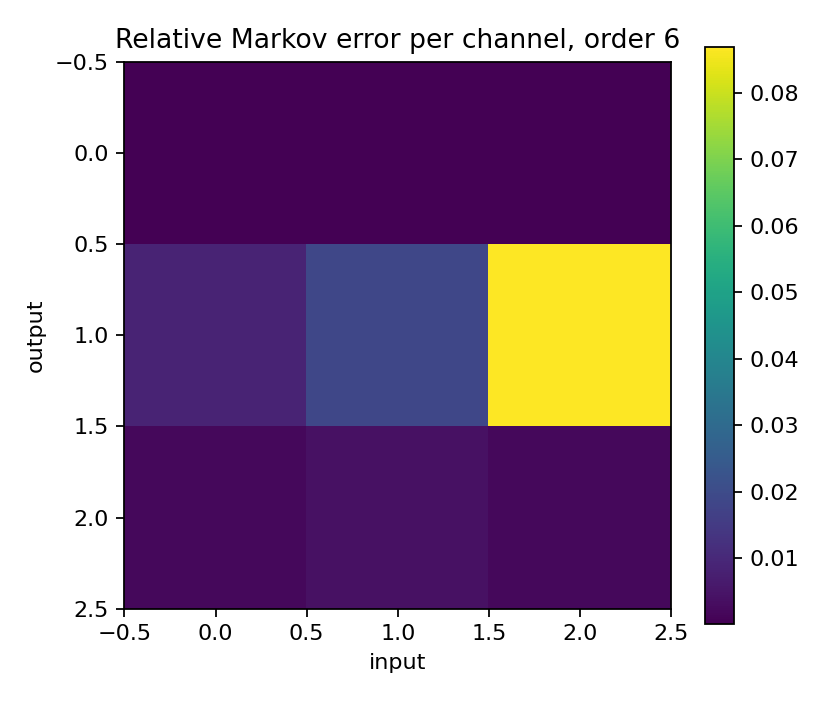
mimo_coupled_error_heatmap.png
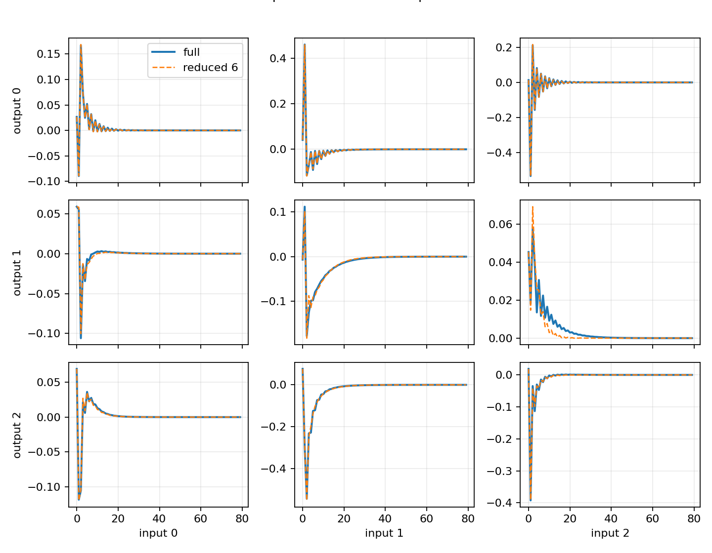
mimo_coupled_markov_responses.png
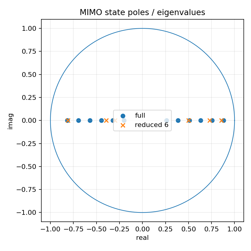
mimo_coupled_state_poles.png
Generated data files
Source code
  1"""Tutorial: coupled MIMO finite-Hankel model reduction.
  2
  3The diagonal MIMO tutorial shows that independent SISO filters are a special
  4case of MIMO.  This tutorial moves to the genuinely coupled case: every input
  5can affect every output through a shared stable state-space model.
  6
  7The reducer works with Markov matrices, builds a finite block-Hankel matrix, and
  8returns a reduced state-space realization.  This is the reference MIMO finite-section baseline and is separate from
  9matrix AAK/Nehari optimality claims.
 10"""
 11
 12from __future__ import annotations
 13
 14import csv
 15import os
 16from pathlib import Path
 17
 18import numpy as np
 19
 20import lattice_dsp as ld
 21
 22
 23def artifact_dir() -> Path:
 24    path = Path(os.environ.get("LATTICE_DSP_ARTIFACT_DIR", "reports/example-artifacts"))
 25    path.mkdir(parents=True, exist_ok=True)
 26    return path
 27
 28
 29def coupled_state_space(order: int = 12, outputs: int = 3, inputs: int = 3, seed: int = 31):
 30    """Return a stable, visibly coupled MIMO state-space system.
 31
 32    The construction uses a random orthogonal basis and deliberately dense B/C/D
 33    matrices so off-diagonal input-output channels are nonzero.  The eigenvalues
 34    of A are inside the unit disk by construction.
 35    """
 36
 37    rng = np.random.default_rng(seed)
 38    q, _ = np.linalg.qr(rng.normal(size=(order, order)))
 39    radii = np.linspace(0.88, 0.20, order)
 40    signs = np.where(np.arange(order) % 2 == 0, 1.0, -1.0)
 41    A = q @ np.diag(signs * radii) @ q.T
 42
 43    B = 0.32 * rng.normal(size=(order, inputs))
 44    C = 0.32 * rng.normal(size=(outputs, order))
 45    D = 0.03 * rng.normal(size=(outputs, inputs))
 46
 47    # Add deterministic cross-channel structure so the system is not close to diagonal.
 48    if outputs == inputs:
 49        D += 0.04 * (np.ones((outputs, inputs)) - np.eye(outputs))
 50    return A, B, C, D
 51
 52
 53def state_spectral_radius(A) -> float:
 54    A = np.asarray(A, dtype=float)
 55    if A.size == 0:
 56        return 0.0
 57    return float(np.max(np.abs(np.linalg.eigvals(A))))
 58
 59
 60def state_space_process_python(A, B, C, D, x):
 61    A = np.asarray(A, dtype=float)
 62    B = np.asarray(B, dtype=float)
 63    C = np.asarray(C, dtype=float)
 64    D = np.asarray(D, dtype=float)
 65    x = np.asarray(x, dtype=float)
 66
 67    batch, samples, _ = x.shape
 68    n_outputs = D.shape[0]
 69    n_state = A.shape[0]
 70    state = np.zeros((batch, n_state), dtype=float)
 71    y = np.zeros((batch, samples, n_outputs), dtype=float)
 72
 73    for n in range(samples):
 74        xn = x[:, n, :]
 75        y[:, n, :] = state @ C.T + xn @ D.T
 76        if n_state:
 77            state = state @ A.T + xn @ B.T
 78    return y
 79
 80
 81def state_space_process(A, B, C, D, x):
 82    """Process batched MIMO signals through a state-space model.
 83
 84    The installed package exposes a compiled C++/OpenMP processor.  The small
 85    Python fallback keeps the tutorial readable if someone opens it against an
 86    older local extension before rebuilding.
 87    """
 88
 89    compiled = getattr(ld, "mimo_state_space_process_batch", None)
 90    if compiled is None:
 91        return state_space_process_python(A, B, C, D, x)
 92    return compiled(A, B, C, D, x)
 93
 94
 95def relative_channel_error(reference, estimate):
 96    """Return per-output/input relative Markov errors."""
 97
 98    reference = np.asarray(reference, dtype=float)
 99    estimate = np.asarray(estimate, dtype=float)
100    num = np.sum((reference - estimate) ** 2, axis=0)
101    den = np.sum(reference**2, axis=0) + 1e-30
102    return num / den
103
104
105def main() -> None:
106    out_dir = artifact_dir()
107
108    full_order = 12
109    inputs = outputs = 3
110    n_markov = 220
111    block_rows = block_cols = 28
112    reduced_orders = [2, 4, 6, 8]
113
114    A, B, C, D = coupled_state_space(full_order, outputs, inputs)
115    markov = ld.mimo_state_space_markov_response(A, B, C, D, n_markov)
116
117    rng = np.random.default_rng(123)
118    x = rng.normal(size=(16, 3000, inputs))
119    y_full = state_space_process(A, B, C, D, x)
120
121    summary = []
122    reduced_markov = {}
123    reduced_outputs = {}
124    reduced_results = {}
125
126    for order in reduced_orders:
127        result = ld.finite_hankel_reduce_mimo(
128            markov,
129            reduced_order=order,
130            block_rows=block_rows,
131            block_cols=block_cols,
132        )
133        approx_markov = ld.mimo_state_space_markov_response(
134            result["A"], result["B"], result["C"], result["D"], n_markov
135        )
136        y_reduced = state_space_process(result["A"], result["B"], result["C"], result["D"], x)
137
138        rel_markov = float(np.sum((markov - approx_markov) ** 2) / (np.sum(markov**2) + 1e-30))
139        rel_output = float(np.sum((y_full - y_reduced) ** 2) / (np.sum(y_full**2) + 1e-30))
140        output_snr = float(10.0 * np.log10(1.0 / max(rel_output, 1e-300)))
141        coupling_error = relative_channel_error(markov, approx_markov)
142
143        reduced_markov[order] = approx_markov
144        reduced_outputs[order] = y_reduced
145        reduced_results[order] = result
146        summary.append(
147            {
148                "order": order,
149                "stable": bool(result["stable"]),
150                "state_radius": state_spectral_radius(result["A"]),
151                "retained_hankel_energy": float(result["retained_hankel_energy"]),
152                "relative_markov_error": rel_markov,
153                "relative_output_error": rel_output,
154                "output_snr_db": output_snr,
155                "max_channel_markov_error": float(np.max(coupling_error)),
156            }
157        )
158
159    csv_path = out_dir / "mimo_coupled_model_reduction_summary.csv"
160    with csv_path.open("w", newline="", encoding="utf-8") as f:
161        writer = csv.DictWriter(f, fieldnames=list(summary[0]))
162        writer.writeheader()
163        writer.writerows(summary)
164
165    hsv = np.asarray(reduced_results[reduced_orders[-1]]["hankel_singular_values"], dtype=float)
166    print("full state order:", full_order)
167    print("inputs:", inputs, "outputs:", outputs)
168    print("full state spectral radius:", f"{state_spectral_radius(A):.4f}")
169    print("block Hankel matrix:", f"{block_rows * outputs} x {block_cols * inputs}")
170    print("leading block-Hankel singular values:", [round(float(v), 6) for v in hsv[:10]])
171    for row in summary:
172        print(
173            "order={order}: stable={stable}, radius={state_radius:.4f}, retained={retained_hankel_energy:.6f}, "
174            "markov_error={relative_markov_error:.3e}, output_snr={output_snr_db:.2f} dB".format(
175                **row
176            )
177        )
178    print(f"wrote {csv_path}")
179
180    try:
181        import matplotlib.pyplot as plt
182    except Exception:
183        print("matplotlib is not installed; skipped figures")
184        return
185
186    fig, ax = plt.subplots(figsize=(8.5, 4.5))
187    idx = np.arange(1, min(35, hsv.size) + 1)
188    ax.semilogy(idx, hsv[: idx.size], marker="o")
189    ax.set_title("Coupled MIMO block-Hankel singular values")
190    ax.set_xlabel("index")
191    ax.set_ylabel("singular value")
192    ax.grid(True, alpha=0.3)
193    fig.tight_layout()
194    fig_path = out_dir / "mimo_coupled_block_hankel_singular_values.png"
195    fig.savefig(fig_path, dpi=160)
196    print(f"wrote {fig_path}")
197
198    selected_order = 6
199    fig2, axes = plt.subplots(outputs, inputs, figsize=(9, 7), sharex=True)
200    t = np.arange(80)
201    for y in range(outputs):
202        for u in range(inputs):
203            ax = axes[y, u]
204            ax.plot(t, markov[: t.size, y, u], linewidth=1.8, label="full")
205            ax.plot(
206                t,
207                reduced_markov[selected_order][: t.size, y, u],
208                "--",
209                linewidth=1.2,
210                label=f"reduced {selected_order}",
211            )
212            ax.grid(True, alpha=0.25)
213            if y == outputs - 1:
214                ax.set_xlabel(f"input {u}")
215            if u == 0:
216                ax.set_ylabel(f"output {y}")
217    axes[0, 0].legend(loc="upper right")
218    fig2.suptitle("Coupled MIMO Markov responses", y=1.02)
219    fig2.tight_layout()
220    fig2_path = out_dir / "mimo_coupled_markov_responses.png"
221    fig2.savefig(fig2_path, dpi=160)
222    print(f"wrote {fig2_path}")
223
224    err = relative_channel_error(markov, reduced_markov[selected_order])
225    fig3, ax3 = plt.subplots(figsize=(5.2, 4.4))
226    im = ax3.imshow(err)
227    ax3.set_title(f"Relative Markov error per channel, order {selected_order}")
228    ax3.set_xlabel("input")
229    ax3.set_ylabel("output")
230    fig3.colorbar(im, ax=ax3)
231    fig3.tight_layout()
232    fig3_path = out_dir / "mimo_coupled_error_heatmap.png"
233    fig3.savefig(fig3_path, dpi=160)
234    print(f"wrote {fig3_path}")
235
236    fig4, ax4 = plt.subplots(figsize=(5.2, 5.2))
237    theta = np.linspace(0, 2 * np.pi, 400)
238    ax4.plot(np.cos(theta), np.sin(theta), linewidth=1.0)
239    ax4.scatter(
240        np.real(np.linalg.eigvals(A)), np.imag(np.linalg.eigvals(A)), marker="o", label="full"
241    )
242    ax4.scatter(
243        np.real(np.linalg.eigvals(reduced_results[selected_order]["A"])),
244        np.imag(np.linalg.eigvals(reduced_results[selected_order]["A"])),
245        marker="x",
246        label=f"reduced {selected_order}",
247    )
248    ax4.set_aspect("equal", adjustable="box")
249    ax4.set_title("MIMO state poles / eigenvalues")
250    ax4.set_xlabel("real")
251    ax4.set_ylabel("imag")
252    ax4.legend()
253    ax4.grid(True, alpha=0.25)
254    fig4.tight_layout()
255    fig4_path = out_dir / "mimo_coupled_state_poles.png"
256    fig4.savefig(fig4_path, dpi=160)
257    print(f"wrote {fig4_path}")
258
259
260if __name__ == "__main__":
261    main()