Periodogram versus AR spectral estimates

Tutorial goal

Compare a windowed periodogram with Levinson and Burg AR spectra on a noisy two-tone signal.

Note

New to the terminology? See the lattice DSP concept map and the causality/data-use guide for how online, offline, block, and MIMO examples should be read.

Context

This tutorial introduces the visual diagnostics that make the AR tools easier to interpret. The periodogram is a direct Fourier estimate; AR spectra are model-based and can sharpen peaks, but they also depend on the chosen model order.

Key idea and equations

The periodogram estimates power directly from the DFT,

\[\hat S_{\mathrm{per}}(\omega)=|\mathrm{DFT}\{w[n]x[n]\}|^2,\]

while an AR spectrum uses

\[\hat S_{\mathrm{AR}}(\omega) \propto \frac{1}{|\hat A(e^{j\omega})|^2}.\]

How to read the result

The vertical dotted lines mark the true tones. Compare how broad the periodogram peaks are with the sharper AR curves, and check the CSV for numeric values.

Run command

python examples/periodogram_vs_ar_spectrum.py

Run status

Return code: 0

Captured stdout

true tone frequencies: [0.18, 0.228]
AR model order: 18
periodogram peak estimates: [0.1799, 0.228]
Levinson AR peak estimates: [0.1794, 0.2283]
Burg AR peak estimates: [0.1797, 0.2288]

Figures

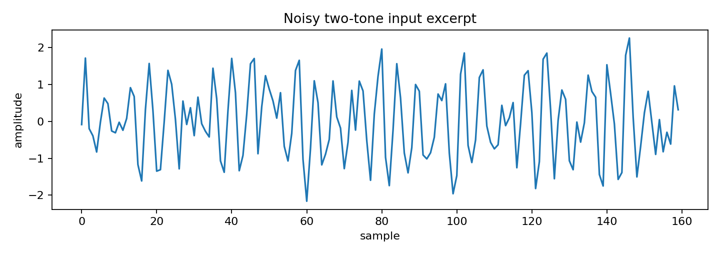
periodogram_vs_ar_signal.png

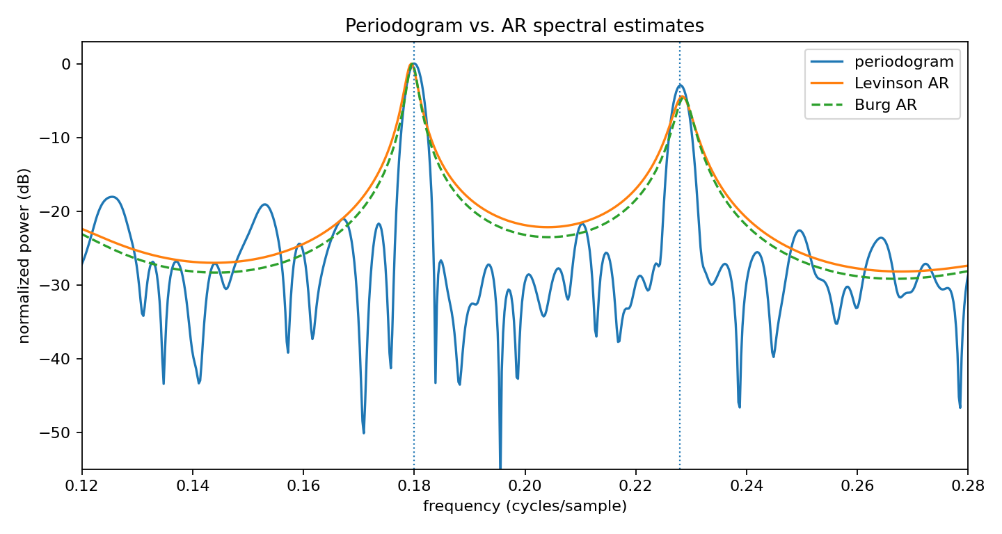
periodogram_vs_ar_spectrum.png

Generated data files

• periodogram_vs_ar_spectrum.csv

Source code

"""Tutorial: compare a periodogram with AR spectral estimates.

The signal contains two nearby sinusoidal components plus white noise.  A
periodogram is a direct Fourier-domain power estimate, while AR spectra fit an
all-pole model and then evaluate its frequency response.  The example writes a
comparison plot and a CSV file to the configured artifact directory.
"""

from __future__ import annotations

import csv
import os
from pathlib import Path

import numpy as np

from lattice_dsp import autocorrelation, burg_denominator, levinson_durbin_denominator


def artifact_dir() -> Path:
    path = Path(os.environ.get("LATTICE_DSP_ARTIFACT_DIR", "reports/example-artifacts"))
    path.mkdir(parents=True, exist_ok=True)
    return path


def db_normalized(power: np.ndarray) -> np.ndarray:
    power = np.maximum(np.asarray(power, dtype=float), 1e-18)
    return 10.0 * np.log10(power / np.max(power))


def periodogram(x: np.ndarray, n_fft: int) -> tuple[np.ndarray, np.ndarray]:
    window = np.hanning(x.size)
    spectrum = np.fft.rfft(window * x, n=n_fft)
    scale = np.sum(window**2)
    power = np.abs(spectrum) ** 2 / max(scale, 1e-12)
    freq = np.fft.rfftfreq(n_fft, d=1.0)
    return freq, power


def ar_spectrum(denominator: np.ndarray, n_fft: int) -> tuple[np.ndarray, np.ndarray]:
    freq = np.linspace(0.0, 0.5, n_fft // 2 + 1)
    z = np.exp(-2j * np.pi * freq)
    a = np.zeros_like(z, dtype=complex)
    for i, coef in enumerate(denominator):
        a += float(coef) * z**i
    power = 1.0 / np.maximum(np.abs(a) ** 2, 1e-18)
    return freq, power


def top_peaks(freq: np.ndarray, db: np.ndarray, count: int = 3, guard_bins: int = 8) -> list[float]:
    candidates = db.copy()
    peaks: list[float] = []
    for _ in range(count):
        idx = int(np.argmax(candidates))
        peaks.append(float(freq[idx]))
        lo = max(0, idx - guard_bins)
        hi = min(candidates.size, idx + guard_bins + 1)
        candidates[lo:hi] = -np.inf
    return peaks


def write_csv(path: Path, freq: np.ndarray, columns: dict[str, np.ndarray]) -> None:
    with path.open("w", newline="", encoding="utf-8") as f:
        writer = csv.writer(f)
        writer.writerow(["frequency_cycles_per_sample", *columns])
        for i, value in enumerate(freq):
            writer.writerow([value, *(columns[name][i] for name in columns)])


def main() -> None:
    rng = np.random.default_rng(2026)
    samples = 512
    n = np.arange(samples)
    tones = [0.180, 0.228]
    x = (
        1.0 * np.sin(2.0 * np.pi * tones[0] * n)
        + 0.75 * np.sin(2.0 * np.pi * tones[1] * n + 0.4)
        + 0.45 * rng.normal(size=samples)
    )
    x -= np.mean(x)

    n_fft = 4096
    order = 18
    freq, p_periodogram = periodogram(x, n_fft)

    r = autocorrelation(x, order)
    den_levinson = np.asarray(levinson_durbin_denominator(r, order), dtype=float)
    den_burg = np.asarray(burg_denominator(x, order), dtype=float)

    _, p_levinson = ar_spectrum(den_levinson, n_fft)
    _, p_burg = ar_spectrum(den_burg, n_fft)

    y_periodogram = db_normalized(p_periodogram)
    y_levinson = db_normalized(p_levinson)
    y_burg = db_normalized(p_burg)

    out_dir = artifact_dir()
    csv_path = out_dir / "periodogram_vs_ar_spectrum.csv"
    write_csv(
        csv_path,
        freq,
        {
            "periodogram_db": y_periodogram,
            "levinson_ar_db": y_levinson,
            "burg_ar_db": y_burg,
        },
    )

    print("true tone frequencies:", tones)
    print("AR model order:", order)
    print("periodogram peak estimates:", [round(v, 4) for v in top_peaks(freq, y_periodogram, 2)])
    print("Levinson AR peak estimates:", [round(v, 4) for v in top_peaks(freq, y_levinson, 2)])
    print("Burg AR peak estimates:", [round(v, 4) for v in top_peaks(freq, y_burg, 2)])
    print(f"wrote {csv_path}")

    try:
        import matplotlib.pyplot as plt
    except Exception:
        print("matplotlib is not installed; skipped figures")
        return

    fig, ax = plt.subplots(figsize=(9, 4.8))
    ax.plot(freq, y_periodogram, label="periodogram")
    ax.plot(freq, y_levinson, label="Levinson AR")
    ax.plot(freq, y_burg, linestyle="--", label="Burg AR")
    for tone in tones:
        ax.axvline(tone, linestyle=":", linewidth=1.0)
    ax.set_xlim(0.12, 0.28)
    ax.set_ylim(-55, 3)
    ax.set_title("Periodogram vs. AR spectral estimates")
    ax.set_xlabel("frequency (cycles/sample)")
    ax.set_ylabel("normalized power (dB)")
    ax.legend()
    fig.tight_layout()
    fig_path = out_dir / "periodogram_vs_ar_spectrum.png"
    fig.savefig(fig_path, dpi=160)
    print(f"wrote {fig_path}")

    fig2, ax2 = plt.subplots(figsize=(9, 3.2))
    ax2.plot(n[:160], x[:160])
    ax2.set_title("Noisy two-tone input excerpt")
    ax2.set_xlabel("sample")
    ax2.set_ylabel("amplitude")
    fig2.tight_layout()
    fig2_path = out_dir / "periodogram_vs_ar_signal.png"
    fig2.savefig(fig2_path, dpi=160)
    print(f"wrote {fig2_path}")


if __name__ == "__main__":
    main()