Capon/MVDR spectral estimation

Tutorial goal

Use an inverse-covariance Capon spectrum to resolve nearby tones.

Note

New to the terminology? See the lattice DSP concept map and the causality/data-use guide for how online, offline, block, and MIMO examples should be read.

Context

Capon/MVDR spectra are useful as a high-resolution diagnostic. They are not a replacement for every periodogram or AR model, but they are visually helpful when nearby narrowband components are hard to separate.

Key idea and equations

For steering vector a(ω) and loaded covariance matrix R, the Capon spectrum is

\[\hat S_{\mathrm{Capon}}(\omega)=\frac{1}{a(\omega)^H R^{-1} a(\omega)}.\]

How to read the result

The main figure compares periodogram, AR, and Capon curves. The covariance-eigenvalue plot helps diagnose whether the covariance estimate is well conditioned.

Run command

python examples/capon_spectrum_demo.py

Run status

Return code: 0

Captured stdout

true tone frequencies: [0.21, 0.236]
Capon aperture: 32
AR model order: 20
periodogram peak estimates: [0.21, 0.2361]
Capon peak estimates: [0.2102, 0.2129]
AR peak estimates: [0.209, 0.2373]

Figures

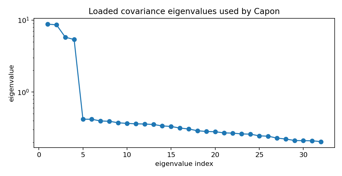
capon_covariance_eigenvalues.png

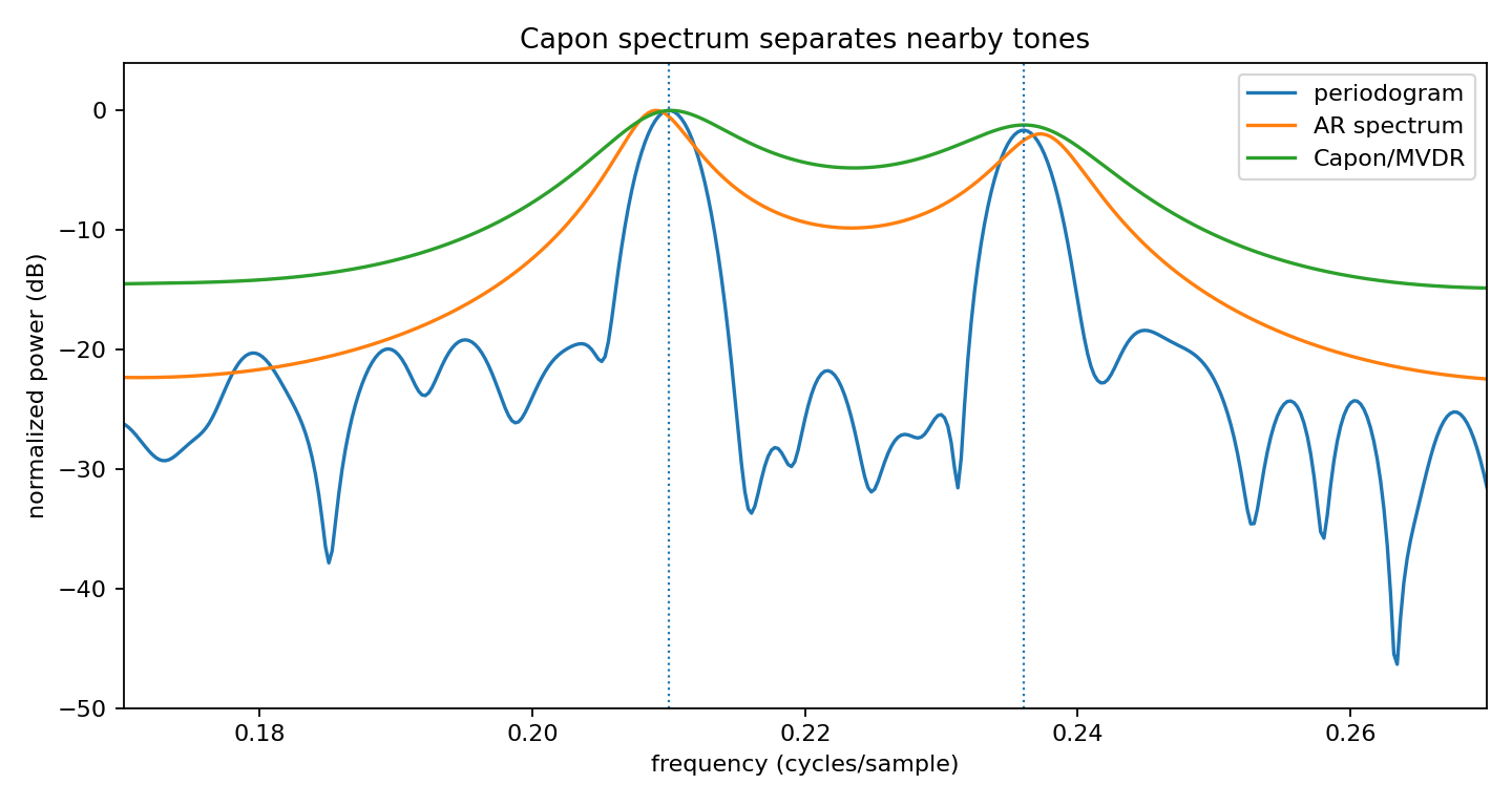
capon_spectrum_demo.png

Generated data files

• capon_spectrum_demo.csv

Source code

"""Tutorial: Capon/MVDR spectral estimation on two close tones.

Capon spectral estimation uses an inverse covariance matrix to minimize output
power subject to unit response at the frequency being tested.  This makes it a
useful high-resolution diagnostic when a periodogram smears together nearby
sinusoids.
"""

from __future__ import annotations

import csv
import os
from pathlib import Path

import numpy as np

from lattice_dsp import autocorrelation, levinson_durbin_denominator


def artifact_dir() -> Path:
    path = Path(os.environ.get("LATTICE_DSP_ARTIFACT_DIR", "reports/example-artifacts"))
    path.mkdir(parents=True, exist_ok=True)
    return path


def db_normalized(power: np.ndarray) -> np.ndarray:
    power = np.maximum(np.asarray(power, dtype=float), 1e-18)
    return 10.0 * np.log10(power / np.max(power))


def periodogram(x: np.ndarray, n_fft: int) -> tuple[np.ndarray, np.ndarray]:
    window = np.hanning(x.size)
    spectrum = np.fft.rfft(window * x, n=n_fft)
    power = np.abs(spectrum) ** 2 / max(np.sum(window**2), 1e-12)
    return np.fft.rfftfreq(n_fft, d=1.0), power


def covariance_from_windows(x: np.ndarray, aperture: int) -> np.ndarray:
    windows = np.lib.stride_tricks.sliding_window_view(x, aperture)
    # One row per window.  Complex dtype keeps the formula general.
    X = windows.astype(complex)
    R = (X.conj().T @ X) / X.shape[0]
    loading = 1e-3 * float(np.trace(R).real) / aperture
    return R + loading * np.eye(aperture)


def capon_spectrum(x: np.ndarray, aperture: int, freq: np.ndarray) -> np.ndarray:
    R = covariance_from_windows(x, aperture)
    Rinv = np.linalg.pinv(R)
    n = np.arange(aperture)
    power = np.empty_like(freq, dtype=float)
    for i, f in enumerate(freq):
        steering = np.exp(-2j * np.pi * f * n)
        denom = np.vdot(steering, Rinv @ steering).real
        power[i] = 1.0 / max(denom, 1e-18)
    return power


def ar_spectrum(denominator: np.ndarray, freq: np.ndarray) -> np.ndarray:
    z = np.exp(-2j * np.pi * freq)
    a = np.zeros_like(z, dtype=complex)
    for i, coef in enumerate(denominator):
        a += float(coef) * z**i
    return 1.0 / np.maximum(np.abs(a) ** 2, 1e-18)


def top_peaks(
    freq: np.ndarray, db: np.ndarray, count: int = 2, guard_bins: int = 10
) -> list[float]:
    candidates = db.copy()
    peaks: list[float] = []
    for _ in range(count):
        idx = int(np.argmax(candidates))
        peaks.append(float(freq[idx]))
        lo = max(0, idx - guard_bins)
        hi = min(candidates.size, idx + guard_bins + 1)
        candidates[lo:hi] = -np.inf
    return peaks


def write_csv(path: Path, freq: np.ndarray, columns: dict[str, np.ndarray]) -> None:
    with path.open("w", newline="", encoding="utf-8") as f:
        writer = csv.writer(f)
        writer.writerow(["frequency_cycles_per_sample", *columns])
        for i, value in enumerate(freq):
            writer.writerow([value, *(columns[name][i] for name in columns)])


def main() -> None:
    rng = np.random.default_rng(314)
    samples = 384
    n = np.arange(samples)
    tones = [0.210, 0.236]
    x = (
        np.sin(2.0 * np.pi * tones[0] * n)
        + 0.9 * np.sin(2.0 * np.pi * tones[1] * n + 0.8)
        + 0.55 * rng.normal(size=samples)
    )
    x -= np.mean(x)

    n_fft = 4096
    freq, p_periodogram = periodogram(x, n_fft)
    aperture = 32
    p_capon = capon_spectrum(x, aperture, freq)

    order = 20
    r = autocorrelation(x, order)
    den = np.asarray(levinson_durbin_denominator(r, order), dtype=float)
    p_ar = ar_spectrum(den, freq)

    y_periodogram = db_normalized(p_periodogram)
    y_capon = db_normalized(p_capon)
    y_ar = db_normalized(p_ar)

    out_dir = artifact_dir()
    csv_path = out_dir / "capon_spectrum_demo.csv"
    write_csv(
        csv_path,
        freq,
        {
            "periodogram_db": y_periodogram,
            "capon_db": y_capon,
            "ar_db": y_ar,
        },
    )

    print("true tone frequencies:", tones)
    print("Capon aperture:", aperture)
    print("AR model order:", order)
    print("periodogram peak estimates:", [round(v, 4) for v in top_peaks(freq, y_periodogram)])
    print("Capon peak estimates:", [round(v, 4) for v in top_peaks(freq, y_capon)])
    print("AR peak estimates:", [round(v, 4) for v in top_peaks(freq, y_ar)])
    print(f"wrote {csv_path}")

    try:
        import matplotlib.pyplot as plt
    except Exception:
        print("matplotlib is not installed; skipped figures")
        return

    fig, ax = plt.subplots(figsize=(9, 4.8))
    ax.plot(freq, y_periodogram, label="periodogram")
    ax.plot(freq, y_ar, label="AR spectrum")
    ax.plot(freq, y_capon, label="Capon/MVDR")
    for tone in tones:
        ax.axvline(tone, linestyle=":", linewidth=1.0)
    ax.set_xlim(0.17, 0.27)
    ax.set_ylim(-50, 4)
    ax.set_title("Capon spectrum separates nearby tones")
    ax.set_xlabel("frequency (cycles/sample)")
    ax.set_ylabel("normalized power (dB)")
    ax.legend()
    fig.tight_layout()
    fig_path = out_dir / "capon_spectrum_demo.png"
    fig.savefig(fig_path, dpi=160)
    print(f"wrote {fig_path}")

    eigvals = np.linalg.eigvalsh(covariance_from_windows(x, aperture))
    fig2, ax2 = plt.subplots(figsize=(7, 3.6))
    ax2.semilogy(np.arange(1, eigvals.size + 1), np.sort(eigvals)[::-1], marker="o")
    ax2.set_title("Loaded covariance eigenvalues used by Capon")
    ax2.set_xlabel("eigenvalue index")
    ax2.set_ylabel("eigenvalue")
    fig2.tight_layout()
    fig2_path = out_dir / "capon_covariance_eigenvalues.png"
    fig2.savefig(fig2_path, dpi=160)
    print(f"wrote {fig2_path}")


if __name__ == "__main__":
    main()